
티스토리 뷰
지난 글에서는( 2023.02.12 - [Remote Sensing] - AI 모델을 사용한 도시 홍수 취약성 지도 제작(2) ) RF(Random Forest), SVM(Support Vector Machine) 및 ANN(Artificial Neural Network)과 같은 포인트 기반 모델을 사용하여 도시 홍수 취약성을 매핑하기 위한 데이터 세트를 준비했습니다. 이 문서에서는 모델을 개발하고 훈련된 모델을 사용하여 도시 홍수 취약성을 매핑하는 방법을 보여줍니다. 이 일련의 기사는 Geomatics, Natural Hazards and Risk에 게시된 " Towards urban flood susceptibility mapping using data-driven models in Berlin, Germany " 논문을 파이썬 코드로 요약하고 설명합니다 .
홍수 취약성을 매핑하기 위해 신뢰할 수 있는 홍수 인벤토리를 수집하는 것은 어려운 일입니다(예: Termeh et al., 2018은 5737km2의 지역에서 53개의 침수 위치를 수집했습니다. Choubin et al., 2019 : 126km2의 51개 위치; Zhao et al. , 2020: 131km2에 216개소). 새로운 연구에 따르면 기계 학습 모델은 작은 데이터 세트에 대한 딥 러닝 모델보다 성능이 뛰어났습니다(Grinsztaj et al., 2022; Shwartz-Ziv and Armon 2022). 따라서 기계 학습 모델이 딥 러닝 모델보다 홍수 감수성에 더 적합하다는 것은 논리적입니다.
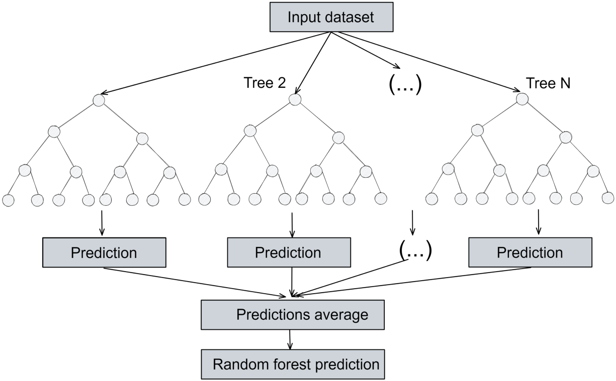
랜덤 포레스트
랜덤 포레스트 모델은 여러 개별 결정 트리로 구성됩니다. 입력 데이터 세트를 여러 하위 샘플로 나누고 각 하위 샘플에 대한 의사 결정 트리 모델을 개발합니다. 최종 결과는 모든 의사 결정 트리 모델의 대다수 결과를 기반으로 추정됩니다(아래 그림 참조).
이제 데이터 세트를 읽고 값이 없는 데이터를 확인하고 삭제합니다. 그런 다음 예측 기능 간의 상관 관계를 살펴봅니다.
<코드 1>
import numpy as np
import cv2
import pandas as pd
from matplotlib import pyplot as plt
import seaborn as sns
import geopandas as gpd

# Read the shapefile or pickle which we created in last article
df=gpd.read_file("points_data.shp")
# df=pd.read_pickle("points_data.pkl") # in case of pickle
df.head()

#check that there is no no data values in the dataset
print(df.isnull().sum())
#df = df.dropna() # use this to remove rows with no data values

#Understand the data
#Here we can see that we have a balanced dataset (equal number of flooded and non flooeded locations
sns.countplot(x="Label", data=df) #0 - Notflooded   B - Flooded


# show the correlation matric for the dataset
corrMatrix = df.corr()
fig, ax = plt.subplots(figsize=(10,10))         # Sample figsize in inches
#sns.heatmap(df.iloc[:, 1:6:], annot=True, linewidths=.5, ax=ax)
sns.heatmap(corrMatrix, annot=True, linewidths=.5, ax=ax)
데이터 프레임은 아래 그림과 같아야 합니다.
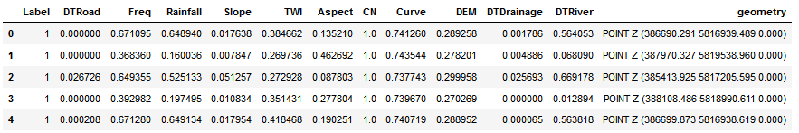
지난 기사에서 준비된 데이터 세트. 표의 값은 인공 신경망과 동일한 데이터 세트를 사용했기 때문에 정규화(0에서 1 사이)됩니다. 그러나 Random Forest에 대한 데이터를 정규화해야 합니다.
데이터 세트는 종속 변수와 독립 변수로 분할되어야 합니다. 종속 변수는 예측해야 하는 변수(열 이름 = 레이블)이고 독립 변수는 예측 기능입니다. 레이블 열의 값은 침수 위치의 경우 1이고 침수되지 않은 위치의 경우 0입니다. 열 도형은 점의 경도와 위도를 나타내며 데이터세트가 원래 점 셰이프파일이기 때문에 데이터세트에 자동으로 포함됩니다.
이제 우리는 두 개의 변수(X와 Y)를 만들 것입니다. Y에는 레이블(종속 변수)이 포함되고 X에는 예측 기능(독립 변수)이 포함됩니다. 그런 다음 데이터 세트(X 및 Y)를 교육(60%), 검증(20%) 및 테스트(20%) 데이터 세트로 분할합니다. 교육 데이터 세트는 모델을 교육하는 데 사용되는 반면 검증 데이터 세트는 초매개변수 조정, 즉 모델 성능을 최적화하는 최상의 매개변수 조합을 추정하는 데 사용됩니다. 마지막으로 테스트 데이터 세트는 모델 성능을 평가하는 데 사용됩니다. 따라서 교육 및 검증 프로세스에 포함되지 않은 데이터 세트에서 모델을 테스트합니다.
<코드 2>
#Define the dependent variable that needs to be predicted (labels)
Y = df["Label"].values

#Define the independent variables. Let's also drop gemotry and label
X = df.drop(labels = ["Label", "geometry"], axis=1)
features_list = list(X.columns)  #List features so we can rank their importance later

#Split data into train (60 %), validate (20 %) and test (20%) to verify accuracy after fitting the model.
# training data is used to train the model
# validation data is used for hyperparameter tuning
# testing data is used to test the model

from sklearn.model_selection import train_test_split
X_train_val, X_test, y_train_val, y_test = train_test_split(X, Y, test_size=0.2,shuffle=True, random_state=42)
X_train, X_val, y_train, y_val = train_test_split(X_train_val, y_train_val, test_size=0.25,shuffle=True, random_state=42)
이제 랜덤 포레스트 모델을 훈련할 수 있습니다. 이 모델은 분류 및 회귀 문제 모두에 사용할 수 있습니다. 그러나 홍수 취약성 매핑은 앞서 언급한 분류 문제입니다. 따라서 sklearn python 모듈의 RandomForestCalssifier를 사용합니다.
<코드 3>
#RANDOM FOREST
from sklearn.ensemble import RandomForestClassifier
model = RandomForestClassifier(random_state = 42) # I am using the default values of the parameters.

# Train the model on training data
model.fit(X_train, y_train)

# make prediction for the test dataset.
prediction = model.predict(X_test)

# The prediction values are either 1 (Flooded) or 0 (Non-Flooded)
prediction

# The AUC is considered one of the best performance indices
# We can plot the curve and calculate it
from sklearn.metrics import plot_roc_curve

ax = plt.gca()
model_disp = plot_roc_curve(model, X_test, y_test, ax=ax, alpha=0.8)
plt.show()
하이퍼파라미터 튜닝에 대해서는 이 문서를 참조하십시오 . 랜덤 포레스트 모델에는 scikit-learn python 모듈에 구현된 내장 기능 중요도 기능이 있습니다. 따라서 어떤 예측 기능이 모델 예측에 영향을 미치는지 추정할 수 있습니다.
<코드 4>
# Estimate the feature importance
feature_imp = pd.Series(model.feature_importances_, index=features_list).sort_values(ascending=False)
print(feature_imp)

# Plot the feature importance
feature_imp.plot.bar()
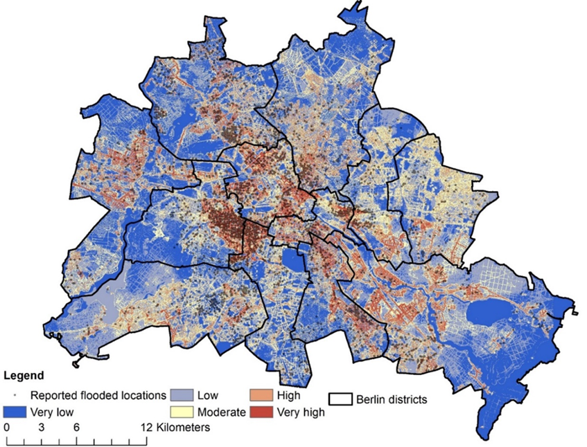
모델 성능에 만족하면 모델을 사용하여 전체 연구 지역에 대한 홍수 취약성을 매핑할 수 있습니다. 훈련된 모델을 사용하여 베를린의 홍수 취약성을 매핑했습니다. 첫째, 지난 글에서 데이터 세트에 대해 수행한 것처럼 전체 연구 영역에 대한 점 모양 파일이 필요합니다 .
<코드 5>
# Read shapefile for the whole study area
df_SA=gpd.read_file("Study_area.shp")
df_SA.head() # make sure that the dataset has the same column arrangement as the training dataset

X_SA= df_SA.drop(labels = ["geometry"], axis=1) # we need to remove all the columns except the predictive features
X_SA.head()

prediction_SA = model.predict(X_SA) # predict if the location is flooded (1) or not flooded (0)

# In order to map the flood susceptibility we need to cacluate the probability of being flooded
prediction_prob=model.predict_proba(X_SA) # This function return an array with lists
# each list has two values [probability of being not flooded , probability of being flooded]

# We need only the probablity of being flooded
# We need to add the value coressponding to each point

df_SA['FSM']= prediction_prob[:,1]
이제 우리는 각 위치의 홍수 민감도가 있는 포인트 셰이프 파일을 갖게 되었습니다. 래스터로 변환해야 합니다. 많은 옵션이 있습니다. ArcMap 또는 QGIS에서 이 단계를 수행하거나 Python에서 계속할 수 있습니다.
<코드 6>
# Save the dataframe tp a shapefile in case of converting the points to raster using QGIS or Arcmap
df_SA.to_file("FSM.shp")

# Converting the point shapefile to raster.
# We will use the model prediction (column FSM in df_SA to make a raster)
from geocube.api.core import make_geocube
import rasterio as rio

out_grid= make_geocube(vector_data=df_SA, measurements=["FSM"], resolution=(-1, 1)) #for most crs negative comes first in resolution
out_grid["FSM"].rio.to_raster("Flood_susceptibility.tif")
최종 결과는 다음과 같은 지도가 됩니다.
참조
- Choubin B, Moradi E, Golshan M, Adamowski J, Sajedi-Hosseini F, Mosavi A. 2019. 다변량 판별 분석, 분류 및 회귀 트리, 지원 벡터 머신을 사용한 홍수 민감성의 앙상블 예측. Sci Total Environ. 651(Pt 2):2087–2096.
- Grinsztajn, L., Oyallon, E., & Varoquaux, G. 2022. 트리 기반 모델이 테이블 형식 데이터에서 여전히 딥 러닝을 능가하는 이유는 무엇입니까? arXiv 프리프린트 arXiv:2207.08815 .
- Shwartz-Ziv, R., & Armon, A. 2022. 표 형식 데이터: 딥 러닝이 필요한 전부는 아닙니다. 정보융합 , 81 , 84–90.
- Termeh SVR, Kornejady A, Pourghasemi HR, Keesstra S. 2018. 적응형 신경 퍼지 추론 시스템 및 메타휴리스틱 알고리즘의 새로운 앙상블을 사용한 홍수 민감성 매핑. Sci Total Environ. 615:438–451.
- Zhao G, Pang B, Xu Z, Peng D, Zuo D. 2020. 컨볼루션 신경망을 기반으로 한 도시 홍수 감수성 평가. J하이드롤. 590:125235.
다음글 (2023.02.20 - [Remote Sensing] - AI 모델을 사용한 도시 홍수 취약성 지도 제작(4))
'Remote Sensing' 카테고리의 다른 글
| AI 모델을 사용한 도시 홍수 취약성 지도 제작(5) (1) | 2023.02.22 |
|---|---|
| AI 모델을 사용한 도시 홍수 취약성 지도 제작(4) (0) | 2023.02.20 |
| 위성사진과 python을 이용하여 토지이용 변화를 정량화 하기 (0) | 2023.02.17 |
| AI 모델을 사용한 도시 홍수 취약성 지도 제작(2) (0) | 2023.02.16 |
| AI 모델을 사용한 도시 홍수 취약성 지도 제작(1) (0) | 2023.02.14 |